How to make formulas. EXCEL formulas with examples

In order to understand how to use this program, you need to consider EXCEL formulas with examples. Excel was created by Microsoft specifically so that users can make any calculations using formulas.

The use of formulas allows you to determine the value of one cell based on the data entered in others. If the data in one cell is changed, then the total value is automatically recalculated. Which is very convenient for carrying out various calculations, including financial ones.

IN Excel program you can perform the most complex mathematical calculations.

In special cells of the file, you need to enter not only data and numbers, but also formulas. At the same time, they must be written correctly, otherwise the subtotals will be incorrect. With the help of the program, the user can perform not only calculations and calculations, but also logical checks.

maximum and minimum values;
averages;
interest;
Student's criterion and much more.

Besides, in excel various text messages, which depend directly on the calculation results.

The main advantage of the program is the ability to convert numerical values and create alternative options, scenarios in which instant results are calculated.

This eliminates the need to enter additional data and parameters.

How to apply simple formulas in the program?

To understand how formulas work in a program, you can first look at easy examples. One such example is the sum of two values. To do this, you need to enter one number in one cell, and another in the second.

For example, in Cell A1 - the number 5, and in cell B1 - 3. In order for the total value to appear in cell A3, you must enter the formula:

SUM(A1;B1).

Each person can determine the sum of the numbers 5 and 3, but you do not need to enter the number in cell C1 yourself, since this is the intent of calculating the formulas. After entering the total appears automatically.

Moreover, if you select cell C1, then the calculation formula is visible in the top line.

If one of the values is changed, the recalculation occurs automatically. For example, when replacing the number 5 in cell B1 with the number 8, you do not need to change the formula, the program will automatically calculate the final value.

In this example, the calculation of total values looks very simple, but it is much more difficult to find the sum of fractional or large numbers.

In Excel, you can perform any arithmetic operation: subtraction "-", division "/", multiplication "*" or addition "+". The formulas specify the type of operation, the coordinates of the cells with the original values, the calculation function.

Any formula must begin with the "=" sign. If you do not put “equal” first, then the program will not be able to give the required value, since the data was entered incorrectly.

Create a formula in Excel

In the above example, the formula =SUM(A1;B1) allows you to determine the sum of two numbers in cells that are located horizontally. The formula starts with the "=" sign. Next is the SUM function. It indicates that the setpoints should be summed.

Cell coordinates are in parentheses. When selecting cells, do not forget to separate them with the sign ";". If you need to find the sum of three numbers, then the formula will look like this:

SUM(A1;B1;C1).

If you need to add 10 or more numbers, then another technique is used that allows you to exclude the selection of each cell. To do this, you just need to specify their range. For example,

SUM(A1:A10). In the figure, the arithmetic operation will look like this:

You can also define the product of these numbers. In the formula, instead of the SUM function, you must select the PRODUCT function and specify a range of cells.

Combined Formulas

The range of cells in the program is specified using the given coordinates of the first and last value. In the formula, they are separated by the sign ":". In addition, Excel has ample opportunities, so the functions here can be combined in any way.

If you need to find the sum of three numbers and multiply the sum by factors of 1.4 or 1.5, based on whether the total number is less than 90 or more.

The problem is solved in the program using one formula that connects several functions and looks like this:

IF(SUM(A1:C1)<90;СУММ(А1:С1)*1,4;СУММ(А1:С1)*1,5).

The example uses two functions, IF and SUM. The first has three arguments:

condition;
right;
wrong.

The task has several conditions. Firstly, the sum of cells in the range A1:C1 is less than 90. If the condition is met that the sum of the range of cells will be 88, then the program will perform the specified action in the 2nd argument of the "IF" function, namely in SUM(A1:C3 )*1.4.

If in this case the number exceeds 90, then the program will calculate the third function - SUM (A1: C1) * 1.5.

Combined formulas are actively used to calculate complex functions. At the same time, their number in one formula can reach 10 or more.

To learn how to perform various calculations and use the Excel program with all its features, you can use the tutorial, which can be purchased or found on the Internet.

Built-in program functions

Excel has functions for all occasions. Their use is necessary for solving various problems at work, study. Some of them can be used only once, while others may not be needed. But there are a number of features that are used regularly.

If you select the “formulas” section in the main menu, then all known functions are concentrated here, including financial, engineering, and analytical ones. In order to select, you should select the item "insert function".

The same operation can be performed using the keyboard combination - Shift + F3 ( earlier we wrote about Excel hotkeys). If you place the mouse cursor on any cell and click on the “select function” item, the function wizard appears.

With its help, you can find the necessary formula as quickly as possible. To do this, you can enter its name, use the category.

Excel is very convenient and easy to use. All functions are divided into categories. If the category of the required function is known, then its selection is carried out according to it.

If the function is unknown to the user, then he can set the category "full alphabetical list".

For example, given the task, find the function SUMIFS. To do this, go to the category of mathematical functions and find the one you need there.

VLOOKUP function

Using the VLOOKUP function, you can extract the necessary information from the tables. The essence of vertical lookup is to look for the value in the leftmost column of the given range.

After that, the total value is returned from the cell, which is located at the intersection of the selected row and column.

The calculation of the VLOOKUP can be seen in the example, which lists the names. The task is to find the last name by the given number.

Applying the VLOOKUP function

The formula shows that the first argument of the function is cell C1. The second argument A1:B10 is the range to search. The third argument is the index number of the column from which to return the result.

Calculating a given last name using the VLOOKUP function

In addition, you can search for the last name even if some sequence numbers are missing. If you try to find the last name from a non-existent number, the formula will not give an error, but will give the correct result.

Search for a last name with missing numbers

This phenomenon is explained by the fact that the VLOOKUP function has a fourth argument, with which you can set the interval view. It has only two values - "false" or "true". If no argument is given, it defaults to true.

Rounding Numbers with Functions

The functions of the program allow you to accurately round any fractional number up or down. And the resulting value can be used in calculations in other formulas.

The number is rounded using the ROUNDUP formula. To do this, you need to fill in the cell. The first argument is 76.375 and the second is 0.

Rounding a number with a formula

In this case, the number has been rounded up. To round a value down, select the ROUNDDOWN function. Rounding occurs to an integer. In our case, up to 77 or 76.

Functions and formulas in Excel help to simplify any calculations. With the help of a spreadsheet, you can complete tasks in higher mathematics. The program is most actively used by designers, entrepreneurs, as well as students.

You can create a simple formula for adding, subtracting, multiplying, and dividing numeric values on a worksheet. Simple formulas always start with an equals sign ( = ), followed by constants, i.e. numeric values, and calculation operators, such as plus ( + ), minus ( - ), asterisk ( * ) and forward slash ( / ).

As an example, consider a simple formula.

Select the cell in the worksheet where you want to enter the formula.

Enter = (equal sign), followed by constants and operators (up to 8192 characters) to be used in the calculation.

In our example, enter =1+1 .

Notes:

Instead of entering constants in a formula, you can select the cells with the desired values and enter operators between them.

In accordance with the standard order of mathematical operations, multiplication and division are performed before addition and subtraction.

Press key ENTER(Windows) or return(Mac).

Consider another version of a simple formula. Enter =5+2*3 in another cell and press the key ENTER or return. Excel will multiply the last two numbers and add the first number to the result of the multiplication.

Using AutoSum

You can use the AutoSum button to quickly add numbers in a column or row. Select the cell next to the numbers you want to add, click the button AutoSum tab home, and then press the key ENTER(Windows) or return(Mac).

When you press the button AutoSum, Excel automatically enters the formula for summing numbers (which uses the SUM function).

Note: You can also type ALT+= (Windows) or ALT+ += (Mac) in a cell and Excel will automatically insert the SUM function.

Example: To add up the numbers for January in the Entertainment budget, select cell B7, which is directly below the column of numbers. Then press the button AutoSum. A formula appears in cell B7, and Excel highlights the cells that are summed up.

To display the result (95.94) in cell B7, press Enter. The formula also appears in the formula bar at the top of the Excel window.

Notes:

To add the numbers in a column, select the cell below the last number in the column. To add the numbers in a row, select the first cell on the right.

Once you create a formula, you can copy it to other cells instead of typing it over and over again. For example, if you copy a formula from cell B7 to cell C7, the formula in cell C7 will automatically adjust to the new location and calculate the numbers in cells C3:C6.

In addition, you can use the AutoSum feature on multiple cells at once. For example, you can select cells B7 and C7, click the button AutoSum and sum two columns at the same time.

Copy the data from the table below and paste it into cell A1 of a new Excel sheet. Change the width of the columns, if necessary, to see all the data.

Note: To make these formulas output the result, select them and press the F2 key, and then - ENTER(Windows) or return(Mac).

Data


Formula	Description	Result
	Sum of values in cells A1 and A2
	Difference of values in cells A1 and A2
	Quotient of the values in cells A1 and A2
	The product of the values in cells A1 and A2
	The value in cell A1 to the power specified in cell A2
Formula	Description	Result

In the second part of the Excel 2010 Beginner series, you'll learn how to link table cells with math formulas, add rows and columns to an existing table, learn about the AutoComplete feature, and more.

Introduction

In the first part of the "Excel 2010 for Beginners" series, we got acquainted with the very basics of Excel, having learned how to create ordinary tables in it. Strictly speaking, this is a simple matter and of course the possibilities of this program are much wider.

The main advantage of spreadsheets is that individual data cells can be linked together by mathematical formulas. That is, when the value of one of the interconnected cells changes, the data of the others will be recalculated automatically.

In this part, we will see how useful such opportunities can be using the example of the budget expenditure table we have already created, for which we will have to learn how to write simple formulas. We will also get acquainted with the autocomplete function of cells and find out how you can insert additional rows and columns into the table, as well as merge cells in it.

Performing basic arithmetic operations

In addition to creating regular tables, Excel can be used to perform arithmetic operations in them, such as addition, subtraction, multiplication, and division.

To perform calculations in any cell of the table, you must create inside it the simplest formula, which must always begin with an equal sign (=). To specify mathematical operations inside a formula, ordinary arithmetic operators are used:

For example, let's imagine that we need to add two numbers - "12" and "7". Place the mouse cursor in any cell and type the following expression: "=12+7". At the end of the input, press the "Enter" key and the result of the calculation - "19" will be displayed in the cell.

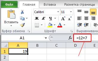
To find out what a cell actually contains - a formula or a number - you need to select it and look at the formula bar - the area immediately above the column names. In our case, it just displays the formula that we just entered.

After carrying out all the operations, pay attention to the result of dividing the numbers 12 by 7, which turned out to be not integer (1.714286) and contains quite a few digits after the decimal point. In most cases, such precision is not required, and such long numbers will only clutter up the table.

To fix this, select the cell with the number for which you want to change the number of decimal places after the decimal point and on the tab home in Group Number select a team Decrease bit depth. Each press of this button removes one character.

To the left of the team Decrease bit depth there is a button that performs the reverse operation - increases the number of decimal places to display more accurate values.

Drawing up formulas

Now let's go back to the budget spending table we created in the first part of this series.

At the moment, it records monthly personal expenses for specific items. For example, you can find out how much was spent in February on food or in March on car maintenance. But the total monthly expenses are not indicated here, although these indicators are the most important for many. Let's correct this situation by adding the line "Monthly expenses" at the bottom of the table and calculate its values.

To calculate the total expense for January in cell B7, you can write the following expression: “=18250+5100+6250+2500+3300” and press Enter, after which you will see the result of the calculation. This is an example of the application of the simplest formula, the compilation of which is no different from calculations on a calculator. Unless the equal sign is placed at the beginning of the expression, and not at the end.

Now imagine that you made a mistake when specifying the values of one or more expense items. In this case, you will have to adjust not only the data in the cells indicating the expenses, but also the formula for calculating the total expenses. Of course, this is very inconvenient, and therefore in Excel, when formulating formulas, not specific numerical values are often used, but cell addresses and ranges.

With that in mind, let's change our formula for calculating total monthly expenses.

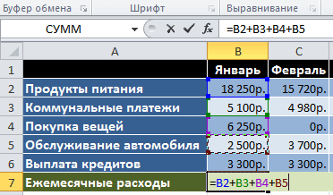
In cell B7, enter an equal sign (=) and ... instead of manually entering the value of cell B2, click on it with the left mouse button. After that, a dotted selection frame will appear around the cell, which shows that its value is included in the formula. Now type a "+" sign and click on cell B3. Next, do the same with cells B4, B5 and B6, and then press the Enter key, after which the same amount value will appear as in the first case.

Select cell B7 again and look at the formula bar. It can be seen that instead of numbers - cell values, the formula contains their addresses. This is a very important point, since we just built the formula not from specific numbers, but from cell values, which can change over time. For example, if you now change the amount of expenses for the purchase of things in January, then the entire monthly total expense will be recalculated automatically. Try it.

Now let's assume that you need to sum up not five values, as in our example, but one hundred or two hundred. As you understand, it is very inconvenient to use the above method of constructing formulas in this case. In this case, it is better to use the special "AutoSum" button, which allows you to calculate the sum of several cells within the same column or row. In Excel, you can count not only the sums of columns, but also rows, so we use it to calculate, for example, total food expenses for six months.

Place the cursor on an empty cell on the side of the required line (in our case it is H2). Then press the button Sum on the bookmark home in Group Editing. Now, let's go back to the table and see what happened.

In the cell we selected, a formula appeared with an interval of cells whose values need to be summed. At the same time, a dotted selection frame appeared again. Only this time it frames not one cell, but the entire range of cells, the sum of which needs to be calculated.

Now let's look at the formula itself. As before, the equals sign comes first, but this time it is followed by function"SUM" is a predefined formula that will add the values of the specified cells. Immediately after the function there are brackets located around the addresses of the cells whose values need to be summed, called formula argument. Please note that the formula does not contain all the addresses of the summed cells, but only the first and last. A colon between them indicates that range cells from B2 to G2.

After pressing Enter, the result will appear in the selected cell, but this button's capabilities Sum do not end. Click on the arrow next to it and a list will open containing functions for calculating the average values (Average), the number of data entered (Number), maximum (Maximum) and minimum (Minimum) values.

So, in our table, we calculated the total expenses for January and the total food expenses for six months. At the same time, they did this in two different ways - first using cell addresses in the formula, and then using functions and ranges. Now, it's time to finish the calculations for the remaining cells, having calculated the total costs for the remaining months and expense items.

Autocomplete

To calculate the remaining amounts, we will use one remarkable feature of the Excel program, which is the ability to automate the process of filling cells with systematized data.

Sometimes in Excel you have to enter similar data of the same type in a certain sequence, such as days of the week, dates, or row numbers. Remember, in the first part of this cycle, in the header of the table, we entered the name of the month in each column separately? In fact, it was completely unnecessary to enter this entire list manually, since the application can in many cases do this for you.

Let's erase all the names of the months in the header of our table, except for the first one. Now select the cell labeled "January" and move the mouse pointer to its lower right corner so that it takes the form of a cross called fill marker. Hold down the left mouse button and drag it to the right.

A tooltip will appear on the screen, which will tell you the value that the program is going to insert in the next cell. In our case, this is "February". As you move the marker down, it will change to the names of other months, which will help you figure out where to stop. After the button is released, the list will be filled in automatically.

Of course, Excel does not always correctly "understand" how to fill in subsequent cells, since the sequences can be quite diverse. Let's imagine that we need to fill a string with even numerical values: 2, 4, 6, 8, and so on. If we enter the number "2" and try to move the autofill marker to the right, it turns out that the program offers, both in the next and in other cells, to insert the value "2" again.

In this case, the application needs to provide a little more data. To do this, in the next cell on the right, enter the number "4". Now select both filled cells and again move the cursor to the lower right corner of the selection area so that it takes the form of a selection marker. By moving the marker down, we see that now the program has understood our sequence and shows the required values in the prompts.

Thus, for complex sequences, before using autocomplete, it is necessary to fill in several cells at once, so that Excel can correctly determine the general algorithm for calculating their values.

Now let's apply this useful feature of the program to our table, no matter what we enter the formulas manually for the remaining cells. First, select the cell with the amount already calculated (B7).

Now "hook" the cursor on the lower right corner of the square and drag the marker to the right to cell G7. After you release the key, the application itself will copy the formula into the marked cells, while automatically changing the addresses of the cells contained in the expression, substituting the correct values.

Moreover, if the marker is moved to the right, as in our case, or down, then the cells will be filled in ascending order, and to the left or up - in descending order.

There is also a way to fill a row with a ribbon. Let's use it to calculate the sums of expenses for all expenditure items (column H).

We select the range to be filled, starting from the cell with the already entered data. Then on the tab home in Group Editing press the button Fill and choose the direction of filling.

Adding Rows, Columns, and Merging Cells

To get more practice in formulating formulas, let's expand our table and at the same time learn a few basic formatting operations. For example, let's add income items to the expenditure side, and then we will calculate possible budget savings.

Suppose that the income part of the table will be located on top of the expenditure part. To do this, we will have to insert a few additional lines. As always, there are two ways to do this: using commands on the ribbon or using the context menu, which is faster and easier.

Click in any cell of the second row with the right mouse button and in the menu that opens, select the command Insert… and then in the window - Add line.

After inserting a row, note the fact that by default it is inserted above the selected row and has the format (cell background color, size settings, text color, etc.) of the row above it.

If you want to change the default formatting, right after pasting, click on the button Add Options, which will automatically appear next to the bottom right corner of the selected cell, and select the option you want.

By a similar method, columns can be inserted into the table, which will be placed to the left of the selected one and individual cells.

By the way, if in the end a row or column ends up in an unnecessary place after insertion, they can easily be deleted. Right-click on any cell belonging to the object to be deleted and in the menu that opens, select the command Delete. Finally, specify what exactly needs to be deleted: a row, a column, or a single cell.

You can use the button on the ribbon for adding operations. Insert located in the group cells on the bookmark home, and for removal, the command of the same name in the same group.

In our case, we need to insert five new rows at the top of the table right after the header. To do this, you can repeat the addition operation several times, or you can use the “F4” key after performing it once, which repeats the most recent operation.

As a result, after inserting five horizontal rows at the top of the table, we bring it to the following form:

We left white unformatted rows in the table on purpose in order to separate the income, expenditure and total parts from each other by writing the appropriate headings in them. But before we do that, we will learn one more operation in Excel - cell merging.

When merging several adjacent cells, one is formed, which can occupy several columns or rows at once. In this case, the name of the merged cell becomes the address of the top maiden cell of the merged range. At any time, you can split a merged cell again, but a cell that has never been merged cannot be split.

When merging cells, only the top left data is saved, while the data of all other merged cells will be deleted. Keep this in mind and it's better to merge first, and only then enter the information.

Let's go back to our table. In order to write headings in white lines, we need only one cell, while now they consist of eight. Let's fix this. Select all eight cells of the second row of the table and on the tab home in Group alignment click the button Merge and center.

After executing the command, all selected cells in the row will be merged into one large cell.

There is an arrow next to the merge button, clicking on which will bring up a menu with additional commands that allow you to: merge cells without center alignment, merge entire groups of cells horizontally and vertically, and also unmerge.

After adding headers, as well as filling in the lines: salary, bonuses and monthly income, our table began to look like this:

Conclusion

In conclusion, let's calculate the last line of our table, using the knowledge gained in this article, the calculation of the cell values of which will occur according to the following formula. In the first month, the balance will consist of the usual difference between the income received for the month and the total expenses in it. But in the second month, we will add the balance of the first month to this difference, since we are calculating savings. Calculations for subsequent months will be carried out according to the same scheme - accumulations for the previous period will be added to the current monthly balance.

Now let's translate these calculations into formulas understandable by Excel. For January (cell B14), the formula is very simple and will look like this: "=B5-B12". But for cell C14 (February), the expression can be written in two different ways: “=(B5-B12)+(C5-C12)” or “=B14+C5-C12”. In the first case, we again calculate the balance of the previous month and then add the balance of the current month to it, and in the second, the already calculated result for the previous month is included in the formula. Of course, using the second option to build a formula in our case is much more preferable. After all, if you follow the logic of the first option, then in the expression for the March calculation there will already be 6 cell addresses, in April - 8, in May - 10, and so on, and when using the second option, there will always be three of them.

To fill in the remaining cells from D14 to G14, we use the ability to automatically fill them, just as we did in the case of the amounts.

By the way, to check the value of the final savings for June, located in cell G14, in cell H14 you can display the difference between the total amount of monthly income (H5) and monthly expenses (H12). As you can see, they must be equal.

As can be seen from the latest calculations, formulas can use not only the addresses of adjacent cells, but also any other, regardless of their location in the document or belonging to a particular table. Moreover, you have the right to link cells located on different sheets of the document and even in different books, but we will talk about this in the next publication.

And here is our final table with the calculations performed:

Now, if you wish, you will be able to continue filling it on your own, inserting both additional items of expenses or income (rows) and adding new months (columns).

In the next article, we will talk in more detail about functions, deal with the concept of relative and absolute links, be sure to master a few more useful table editing elements, and much more.

In order to understand how to use this program, you need to consider EXCEL formulas with examples.

If you place the mouse cursor on any cell and click on the “select function” item, the function wizard appears.

With its help, you can find the necessary formula as quickly as possible. To do this, you can enter its name, use the category.

Excel is very convenient and easy to use. All functions are divided into categories. If the category of the required function is known, then its selection is carried out according to it.

If the function is unknown to the user, then he can set the category "full alphabetical list".

For example, given the task, find the function SUMIFS. To do this, go to the category of mathematical functions and find the one you need there.

VLOOKUP function

Using the VLOOKUP function, you can extract the necessary information from the tables. The essence of vertical lookup is to look for the value in the leftmost column of the given range.

After that, the total value is returned from the cell, which is located at the intersection of the selected row and column.

The calculation of the VLOOKUP can be seen in an example that shows a list of surnames. The task is to find the last name by the given number.

Applying the VLOOKUP function

The formula shows that the first argument of the function is cell C1.

The second argument A1:B10 is the range to search.

The third argument is the index number of the column from which to return the result.

Calculating a given last name using the VLOOKUP function

In addition, you can search for the last name even if some sequence numbers are missing.

If you try to find the last name from a non-existent number, the formula will not give an error, but will give the correct result.

Search for a last name with missing numbers

This phenomenon is explained by the fact that the VLOOKUP function has a fourth argument, with which you can set the interval view.

It has only two values - "false" or "true". If no argument is given, it defaults to true.

Rounding Numbers with Functions

The functions of the program allow you to accurately round any fractional number up or down.

And the resulting value can be used in calculations in other formulas.

The number is rounded using the ROUNDUP formula. To do this, you need to fill in the cell.

The first argument is 76.375 and the second is 0.

Rounding a number with a formula

In this case, the number has been rounded up. To round a value down, select the ROUNDDOWN function.

Rounding occurs to an integer. In our case, up to 77 or 76.

Excel helps to simplify any calculations. With the help of a spreadsheet, you can complete tasks in higher mathematics.

The program is most actively used by designers, entrepreneurs, as well as students.

The whole truth about Microsoft Excel 2007 formulas

EXCEL formulas with examples - Instructions for use

Hello!

Many who do not use Excel - do not even imagine what opportunities this program gives! Just think: automatically add values from one formula to another, search for the desired lines in the text, add by condition, etc. - in general, in fact, a mini-programming language for solving "narrow" tasks (to be honest, for a long time I myself did not consider Excel as a program, and almost did not use it) ...

In this article I want to show a few examples of how you can quickly solve everyday office tasks: add something, subtract something, calculate the sum (including with a condition), substitute values from one table to another, etc. That is, this article will be something like a mini guide on learning the most necessary things for work (more precisely, to start using Excel and feel the full power of this product!).

It is possible that if you had read a similar article 15-17 years ago, I myself would have started using Excel much faster (and would have saved a lot of my time for solving "simple" (note: as I understand now) tasks)...

Note: All screenshots below are from Excel 2016 (as the newest to date).

Many novice users, after starting Excel, ask one strange question: "well, where is the table?". Meanwhile, all the cells that you see after starting the program are one big table!

Now to the main thing: in any cell there can be text, some number, or a formula. For example, the screenshot below shows one illustrative example:

left: Cell (A1) contains the prime number "6". Note that when you select this cell, the formula bar (Fx) just shows the number "6".
right : in cell (C1) it also looks like a simple number "6", but if you select this cell, you will see the formula "=3+3" - this is an important feature in Excel!

Just a number (on the left) and a calculated formula (on the right)

The bottom line is that Excel can count like a calculator if you select some cell, and then write a formula, for example "=3+5+8" (without quotes). You do not need to write the result - Excel will calculate it and display it in the cell (as in cell C1 in the example above)!

But you can write in formulas and add not just numbers, but also numbers already calculated in other cells. In the screenshot below, in cell A1 and B1, the numbers are 5 and 6, respectively. In cell D1, I want to get their sum - you can write the formula in two ways:

first: "=5+6" (not very convenient, imagine that in cell A1 - we also have a number calculated according to some other formula and it changes. You won’t substitute a number instead of 5 every time?!);
the second: "=A1+B1" - and this is the ideal option, just add the value of cells A1 and B1 (regardless of what numbers they contain!)

Add cells that already have numbers

Extending a formula to other cells

In the example above, we added two numbers in column A and B in the first row. But then we have 6 lines, and most often in real problems you need to add numbers in each line! To do this, you can:

on line 2 write the formula "=A2+B2" , on line 3 - "=A3+B3", etc. (this is long and tedious, this option is never used);
select cell D1 (which already has a formula), then move the mouse pointer to the right corner of the cell so that a black cross appears (see screenshot below). Then hold down the left button and stretch the formula to the entire column. Convenient and fast! (Note: You can also use Ctrl+C and Ctrl+V combinations for formulas (copy and paste respectively)).

By the way, pay attention to the fact that Excel itself has substituted formulas in each line. That is, if you now select a cell, say D2, you will see the formula "=A2+B2" (i.e. Excel automatically fills in the formulas and returns the result immediately) .

How to set a constant (a cell that will not change when copying a formula)

Quite often it is required in formulas (when you copy them) that some value does not change. Let's say a simple task: convert prices in dollars into rubles. The cost of the ruble is set in one cell, in my example below it is G2.

Next, in cell E2, the formula "=D2*G2" is written and we get the result. Only now, if we stretch the formula, as we did before, we will not see the result in other lines, because Excel in line 3 will put the formula "D3*G3", in the 4th line: "D4*G4", etc. G2 must remain G2 everywhere...

To do this - just change cell E2 - the formula will look like "=D2*$G$2". Those. dollar sign $ - allows you to set a cell that will not change when you copy the formula (i.e. get a constant, example below)...

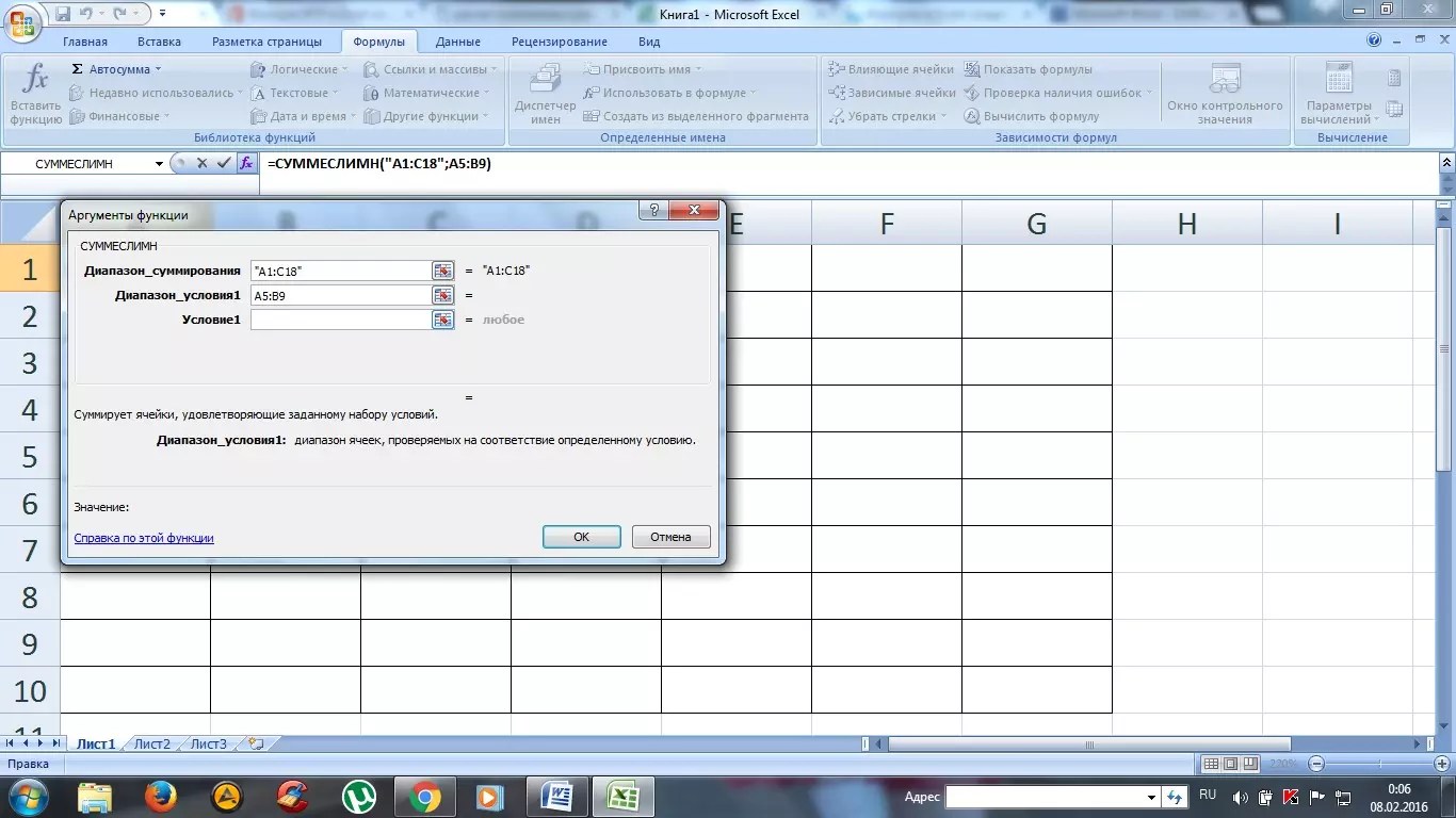
How to calculate the sum (SUM and SUMIFS formulas)

You can, of course, write formulas manually by typing "=A1+B1+C1" and so on. But Excel has faster and more convenient tools.

One of the easiest ways to add up all selected cells is to use the option autosums (Excel will write the formula itself and paste it into the cell).

first select the cells (see screenshot below);
then open the section "Formulas";
The next step is to press the "Autosum" button. Under the cells you selected, the result of the addition will appear;
if you select the cell with the result (in my case, this is the cell E8) - then you will see the formula "=SUM(E2:E7)" .
thus writing the formula "=SUM(xx)", where instead of xx put (or select) any cells, you can read a wide variety of ranges of cells, columns, rows...

Quite often, when working, it is required not just the sum of the entire column, but the sum of certain rows (i.e. selectively). Suppose a simple task: you need to get the amount of profit from some worker (exaggerated, of course, but the example is more than real).

I will use only 7 rows in my table (for clarity), the real table can be much larger. Suppose we need to calculate all the profit that "Sasha" made. What the formula will look like:

"=SUMIFS(F2:F7 ;A2:A7 ;"Sasha") " - (note: pay attention to the quotation marks for the condition - they should be like in the screenshot below, and not as it is written on my blog now). Also note that Excel, when driving in the beginning of a formula (for example, "SUM ..."), itself prompts and substitutes possible options - and there are hundreds of formulas in Excel!;
F2:F7 - this is the range over which the numbers from the cells will be added (summed up);
A2:A7 is the column by which our condition will be checked;
"Sasha" is a condition, those lines in which "Sasha" will be in column A will be added (pay attention to the indicative screenshot below).

Note: there can be several conditions and you can check them in different columns.

How to count the number of rows (with one, two or more conditions)

Quite a typical task: to calculate not the sum in the cells, but the number of rows that satisfy some condition. Well, for example, how many times the name "Sasha" occurs in the table below (see screenshot). Obviously, 2 times (but this is because the table is too small and taken as a good example). How can this be calculated as a formula? Formula:

"=COUNTIF(A2:A7 ,A2 )" - Where:

A2:A7- the range in which lines will be checked and counted;
A2- a condition is set (note that you could write a condition like "Sasha", or you can just specify a cell).

The result is shown on the right side of the screenshot below.

Now imagine a more extended task: you need to count the lines where the name "Sasha" occurs, and where in the AND column there will be the number "6". Looking ahead, I will say that there is only one such line (screen with an example below).

The formula will look like:

=COUNTIFS(A2:A7 ;A2 ;B2:B7 ;"6") (note: pay attention to the quotes - they should be like in the screenshot below, and not like mine), Where:

A2:A7 ;A2- the first range and search condition (similar to the example above);

B2:B7 ;"6"- the second range and the search condition (note that the condition can be specified in different ways: either specify a cell, or simply write text/number in quotes).

How to calculate the percentage of the amount

It's a very common question that I often come across. In general, as far as I can imagine, it occurs most often - due to the fact that people get confused and do not know what percentage is looking for (and in general, they do not understand the topic of interest well (although I myself am not a great mathematician, and yet ...)).

The simplest way, in which it is simply impossible to get confused, is to use the "square" rule, or proportion. The whole essence is shown on the screen below: if you have a total amount, let's say in my example this number is 3060 - cell F8 (i.e. this is 100% profit, and "Sasha" made some part of it, you need to find which ... ).

In proportion, the formula will look like this: =F10*G8/F8(i.e. cross by cross: first we multiply two known numbers diagonally, and then divide by the remaining third number). In principle, using this rule, it is almost impossible to get lost in percentages.

Actually, this concludes this article. I'm not afraid to say that having mastered everything that is written above (and only "heels" of formulas are given here) - you will be able to learn Excel on your own, flip through help, watch, experiment, and analyze. I will say even more, everything that I described above will cover many tasks, and will allow you to solve the most common ones that you often puzzle over (if you don’t know the capabilities of Excel), and you don’t know how to do it faster ...